doi: 10.56294/dm202338
ORIGINAL
Deep Learning Based Analysis of Student Aptitude for Programming at College Freshman Level
Análisis basado en aprendizaje profundo de la aptitud de los estudiantes para la programación en el primer año de universidad universitario
V. Lakshmi Narasimhan1 *, G. Basupi2 *
1Georgia Southern University, USA.
2University of Botswana, Botswana.
Cite as: Simhan L, Basupi G. None Deep Learning Based Analysis of Student Aptitude for Programming at College Freshman Level: None. Data & Metadata. 2023;2:38. https://doi.org/10.56294/dm202338
Submitted: 06-04-2023 Revised: 23-06-2023 Accepted: 14-08-2023 Published: 15-08-2023
Editor: Prof.
Dr. Javier González Argote ![]()
ABSTRACT
Predicting Freshman student’s aptitude for computing is critical for researchers to understand the underlying aptitude for programming. Dataset out of a questionnaire taken from various Senior students in a high school in the city of Kanchipuram, Tamil Nadu, India was used, where the questions related to their social and cultural back- grounds and their experience with computers. Several hypotheses were also generated. The datasets were analyzed using three machine learning algorithms namely, Back- propagation Neural Network (BPN) and Recurrent Neural Network (RNN) (and its variant, Gated Recurrent Network (GNN)) with K-Nearest Neighbor (KNN) used as the classifier. Various models were obtained to validate the under- pinning set of hypotheses clusters. The results show that the BPN model achieved a high degree of accuracies on various metrics in predicting Freshman student’s aptitude for computer programming.
Keywords: Freshman Students; Aptitude for Programming; Machine Learning; K Nearest Neighbor (KNN); Backpropagation Neural Network (BPN); Recurrent Neural Network (RNN); Gated Recurrent Unit (GNN).
RESUMEN
Predecir la aptitud de los estudiantes de primer año para la informática es fundamental para que los investigadores comprendan la aptitud subyacente para la programación. Se utilizó un conjunto de datos procedentes de un cuestionario realizado a varios estudiantes de último curso de un instituto de la ciudad de Kanchipuram, en Tamil Nadu (India), en el que las preguntas se referían a sus antecedentes sociales y culturales y a su experiencia con los ordenadores. También se generaron varias hipótesis. Los conjuntos de datos se analizaron mediante tres algoritmos de aprendizaje automático: la red neuronal de retropropagación (BPN) y la red neuronal recurrente (RNN) (y su variante, la red neuronal recurrente cerrada (GNN)), con el clasificador K-Nearest Neighbor (KNN). Se obtuvieron varios modelos para validar el conjunto de conglomerados de hipótesis. Los resultados muestran que el modelo BPN alcanzó un alto grado de precisión en varias métricas en la predicción de la aptitud de los estudiantes de primer año para la programación de ordenadores.
Palabras clave: Estudiantes de Primer Año; Aptitud para la Programación; Aprendizaje Automático; K Nearest Neighbor (KNN); Backpropagation Neural Network (BPN); Recurrent Neural Network (RNN); Gated Recurrent Unit (GNN).
INTRODUCTION
Computer science programs around the world always have students facing problems with programming courses, such as Programming Principles, Object-Oriented Programming and Data Structures.
Most of the time, students fail later programming courses because of the lack of foundation at Freshmen level and, this has something to do with their aptitude for programing.
In order to help potential applicants of the program to understand the kind of competencies of abstract and logical thinking skills that are needed for computer science programing courses and to help the University admissions office in selecting potential candidates for such courses, a study has been carried out among final year high school students.
A model that helps in predicting student aptitude for programming based on several features was built. Datasets ac- quired through a questionnaire were analyzed using data analytics software, e.g., Python Libraries, PyTorch and TensorFlow.
The model used machine learning to classify the student aptitude for computer programming, which helps in identifying students who are at risk of failing; note that improving the passing rates in introductory courses has a direct impact on retention rate also.
Unlike other studies, which often correlate student’s aptitude to programming to student’s past academic performance, this study considers student’s family background and individual’s interaction with technology also; the authors feel that these are foundational factors in student’s attitude to programming.
The rest of the paper is organized as follows: section 2 describes the problem statement and related literature, while section 3 details the hypotheses and the questionnaire design. Section 4 presents the analysis approach & deep learning algorithms used, while section 5 provides the results of the study.
Problem description & related literature
The literature review has two components, namely, i) those relating to model development and related factors that affect aptitude for programming and ii) the use of machine learning techniques for analyzing student’s aptitude for programming.
Identifying the factors that affect student aptitude to programming can also help us to understand how students learn to program, which in turn can help to plan the needed intervention at an early stage and avoid the risk of student retention in the program. Most of the factors that can be situated with one’s aptitude for computer programming are abstract thinking, logical thinking, mathematical skills, and problem-solving skills.
Some studies indicate that gender plays a role and in this modern age, males do dominant the world of computer Science. Results from several studies show that there is a statistically significant difference in programming performance between male and female students, where male students performed better than their female counterparts.(1)
A key factor that researchers omit is students background, but instead assume that student’s performance is based on their previous grades or such skills as problem solving skills. Psychological and sociological factors play a big part in student’s aptitude for programming and such factors as predictors can be helpful in understanding the process that students go through when learning.(2)
Other studies indicate that just the behavior of a student during lectures and labs play a huge impact towards aptitude for programming – e.g., gestures, outbursts, and other factors including collaboration with other students.(3)
However, these studies lack depth of statistical significance in the larger context of the underlying question. A small amount of literature exists on using machine learning techniques for analyzing student’s aptitude for programming.
Longi(3) details the use of Bayesian network to model the relationship between factors that affect programming performance. Further detailed literature analysis can be obtained from the authors, which due to space limitations has been curtailed, but can be obtained from the authors.
HYPOTHESES & QUESTIONNAIRE DESIGN
In our earlier detailed research work,(4,5) we developed a set of hierarchical hypotheses and corresponding questionnaire for comprehending Freshman aptitude for computer programming – as shown in Appendix–A. They deal with psychological and sociological aspects of student’s views on computing and programming. It is noted that these hypotheses and questionnaire are better suited for Third World countries and rural students in the First World countries, who in general are not exposed to computing and computers much. The questionnaire was distributed to Senior students in a high school in the city of Kanchipuram, Tamil Nadu, India, and a large body of data was collected.
Dataset Description & Analysis Basics
It is noted that the questionnaire (Appendix-A) is in two parts, viz., Part-A and Part-B. Details from the questionnaire were converted into a dataset format, which was further cleaned for any errors; missing values were normalized using mean values. The dataset consisted of 157 instances, with 35 attributes. The Likert Scale was used to rate each of the questions asked and it ranged from 0 to 7, where 0 is none, 1 – 6 being Strongly Disagree to Strongly Agree and 7 being not applicable. Part-A of the dataset deals with students’ biographical backgrounds which are detailed in figure 1 and 2.

Figure 1. Part-A Student-Biographical Information

Figure 2. Dataset Attributes
Part-B of the dataset (figure 3) relates ti students’ programming experience, which is derived from clustering Q1-Q35 from Appendix-A. Each of the questions are evaluated using a Likert scale ranging from 0-7.

Figure 3. Part B Computer-Programming-Experience Dataset based on multiple questions Q1 – Q35, each having a Likert range of 0 – 7
Calculation of Mean, Median, Standard Deviation & Rho Values
This paper focusses on Part-B of the dataset which deals with calculating each of the features Mean, Median, Standard Deviation and RHO (Spearman’s Correlation).

Figure 4. Spearman’s Correlation
Hypotheses Clustering
Appendix-A provides the list of hypotheses (H1-H10) and their grouping of the underlying questions into H0 to H10. Once grouped next was selection of the hypothesis were correlated to generate inferences. In this case C1 represents the correlation of hypotheses H0, H1, H2; C2 represents the correlation of H3, H6, H5; C3 represents the correlation of hypotheses H8, H8.1, H8.2 and, C4 represents the correlation of hypotheses H7, H9 and H10.
ANALYSIS APPROACH & DEEP LEARNING ALGORITHMS USED
Figure 5 presents an overview of the workflow, whereas three different machine learning approaches were selected, namely, BNN and RNN (GRU) along with K-nearest neighbor algorithm for clustering; a brief overview of these techniques are presented in Appendix-B. Further, while data analytics open source libraries such as, PyTorch, WEKA, TensorFlow and RapidMiner are available, TensorFlow was chosen because:
1) it provides excellent functionalities and services when compared to other popular deep learning , 2) has low-level libraries which provides more flexibility and 3) a highly interactive development environment that allows for design-as-you-go flexibility. Agile process model was used to develop Machine Learning based model/s as shown in figure 4.

Figure 5. Overview of Workflow of Machine Learning
ANALYSIS OF RESULTS
The models were evaluated using the performance metrics of accuracy, precision, recall, and F1- score, which are defined as follows:
• Accuracy: characterizes the degree to which a predicted value agrees with an actual value.(6)
• Precision: identifies the probability of a positive test result. High precision values indicate that the probability of the test set being accurately classified is high. In the context of this paper, precision indicates the number of students having aptitude for programming.
• Recall: evaluates the number of true positives of the actual class predicted by the models.
• F1-score: indicates the best performing algorithm.
MODEL IMPLEMENTION SUMMARY
Backpropagation Neural Network (BPN)
With the Backpropagation Neural Network (BPN), the datasets were randomly divided into training and test data in the ratio of 80:20; note that Ward, Peters et al.(7) state that if the size of the training dataset is too small or too large, the performance of the models will be affected.
The output variables are the mean of each of the correlation regression. ADAM optimizer(8) was used for each model instead of the classical stochastic gradient descent procedure to update network weights. ADAM updates all parameters with individual learning rates so that every parameter in the network has a specific learning rate.
Correlation C1 relates to hypotheses H0, H1 and H2 and in this case the model was built with one input layer, two hidden layers and one output layer which took an input dimension of 7, 7 representing 7 features (or questions) based on the three hypotheses. The input layer contains 14 nodes with initial weight being uniform and activation function being Sigmoid.(9) The two hidden layers contain 8 nodes and 4 nodes respectively, both having initial weights being uniform and activation function being Sigmoid, while the output layer has one node.
The first test of the model using the number of epochs set to 100 yielded an accuracy of 37,5 %, as shown in Figure 6. As the number of epochs increased from 100 to 400 and a change in the loss function from binary cross to MSE (Mean Square Error), the prediction accuracy became 94 %; further the use of MSE was better than the binary cross function (figure 7). However, the Loss graph still did not converge, thereby meaning that the model has not reached the stopping criteria. With 900 epochs, the model yielded a prediction accuracy of 93,75 %. Based on the three tests, the loss graph starts converging at approximately 600 epochs. The stopping criteria of this model would possibly be at 600 epochs as anything beyond 900 gives an accuracy of 93,750 % as can be evident from Figure 8; the accuracy remains constant from the 500 epochs and beyond. The corresponding Confusion matrix is shown in figure 9.

Figure 6. Model loss graph

Figure 7. Model Loss Graph for 400 epochs
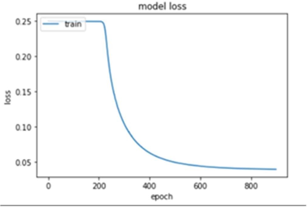
Figure 8. Model Loss Graph for 900 epochs

Figure 9. Confusion Matrix
TP = True Positives = 19; TN = True Negatives = 11; FP = False Positives = 1; FN = False Negatives = 1.
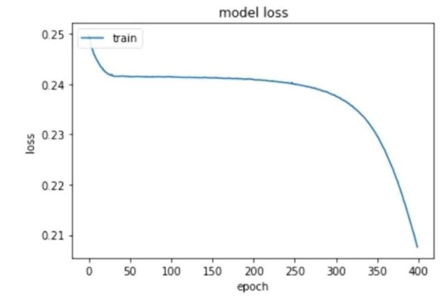
Figure 10. Model Loss Graph for 900 epochs
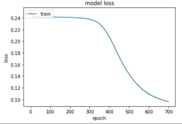
Figure 11. Model Loss Graph for 900 epochs
Correlation 2 relates to hypotheses H3, H5 and H6 and has seven input parameters and the co0orresponding model was built using one input layer, four hidden layers and one output layer. With 400 epochs along with Sigmoid activation function and MSE as the loss function, the model gave a prediction accuracy of 79,411765 %. With an increase in the number of epochs from 400 to 700 (Figures 10 & 11), the model yielded an accuracy of 87,5 %. With 1200 epochs, the Prediction accuracy is 90,625 % and the corresponding confusion matrix as shown in figure 12.
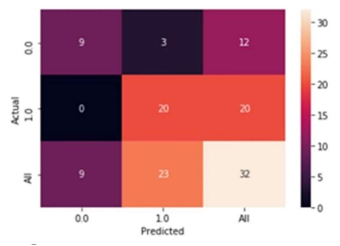
Figure 12. Confusion Matrix
TP = True Positives = 20; TN = True Negatives = 9; FP = False Positives = 3; FN = False Negatives = 0.
Correlation 3 relates to hypotheses H8,0, H8,1 and H8,2 and has seven input parame- ters. The model gave a prediction value of 96,875 % with the test of 800 epochs (Figures 13 & 14) and was declared to yield high prediction accuracy. The Confusion Matrix is shown in figure 15.

Figure 13. Model Loss Graph for 800 epochs

Figure 14. Model Loss Graph for 900 Epochs

Figure 15. Confusion Matrix
TP = True Positives = 22; TN = True Negatives = 9; FP = False Positives = 1; FN = False Negatives = 0.
Correlation 4 relates to hypotheses of H7, H9 and H10 and has nine input parameters and the related model is built using five layers using 900 epochs to train the model, yielding an accuracy of 90,625 % (Figures 16 & 17). The error loss reached the point of convergence with 900 epochs, because of the increase in the number of features. However, even with the addition of an extra layer, the accuracy remained the same hence no further layers are also required. The corresponding confusion matrix is shown in Figure 18.

Figure 16. Model Loss Graph for 700 epochs
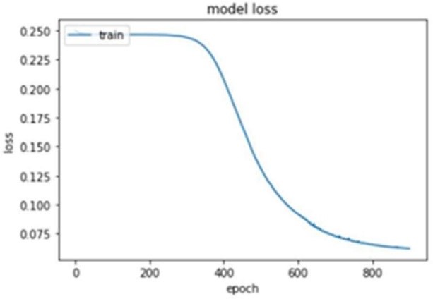
Figure 17. Model Loss Graph for 900 Epochs

Figure 18. Confusion Matrix
TP = True Positives = 18; TN = True Negatives = 11; FP = False Positives = 2; FN = False Negatives = 1.
Gated Recurrent Unit (RGU-ANN)
The datasets were randomly divided into training and test data on the ratio of 80:20. The output variables were the mean of each of the correlation regression and ADAM optimizer was used for each model. All the models were built with activation='Sigmoid' and loss='MSE' and with a batch size of 15.

Figure 19. Model Loss Graph for 700 epochs

Figure 20. Model Loss Graph for 500
Correlation 1 The GRU build model yielded an accuracy of 84,375 % at 700 epochs.
It is evident from Figures 19 & 20 that between 500 to 550 epochs, the model is overfitting and hence the number of epochs is now reduced, which in turn yielded an accuracy of 90,62500 %. The corresponding Confusion Matrix is presented in Figure 21.

Figure 21. Confusion Matrix
TP = True Positives = 19; TN = True Negatives = 10; FP = False Positives = 1; FN = False Negatives = 2
Correlation 2 The model was built using 600 epochs as shown in Figure 22 and the confusion matrix is shown in Figure 23. The model gave a prediction accuracy of 84,37500 %.

Figure 22. Model Loss Graph for 600 epochs

Figure 23. Confusion Matrix
TP = True Positives = 20 ; TN = True Negatives = 7; FP = False Positives = 3; FN = False Negatives = 2.
On Correlation 3, the model yields a prediction accuracy of 96,87500 % with the number of epochs set to 500; the model is declared as having the highest prediction accuracy (Figure 24); the corresponding confusion matrix is shown in Figure 25.

Figure 24. Model Loss Graph for 500 epochs

Figure 25. Confusion Matrix
TP = True Positives = 22; TN = True Negatives = 9; FP = False Positives = 1; FN = False Negatives = 0.
On Correlation 4, the model shown in Figure 26 yields a prediction value of 96.875% at 400 epochs, which was the highest accuracy; the confusion matrix is shown in Figure 27.
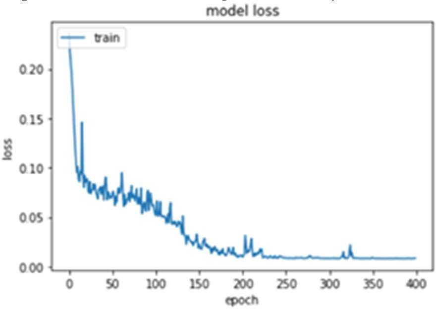
Figure 26. Model Loss Graph for 400 epochs

Figure 27. Confusion Matrix
TP = True Positives = 17 ; TN = True Negatives = 9; FP = False Positives = 3 FN = False Negatives = 3.
K-Nearest Neighbor (KNN)
The machine learning algorithms were applied using hypothesis variables as input to predict aptitude for programming. The KNN was constructed using Python and Kera’s library and the training and test data ratio was set at 80:20. The N-neighbor for each of the model was set to 5; note that the rule of thumb says K = Square Root of N divided by 2, where N is the number of samples in the training set.
For correlation 1, the model yields the best prediction accuracy of 84,375 % at 5 nearest neighbors; the corresponding confusion matrix is shown in Figure 28.
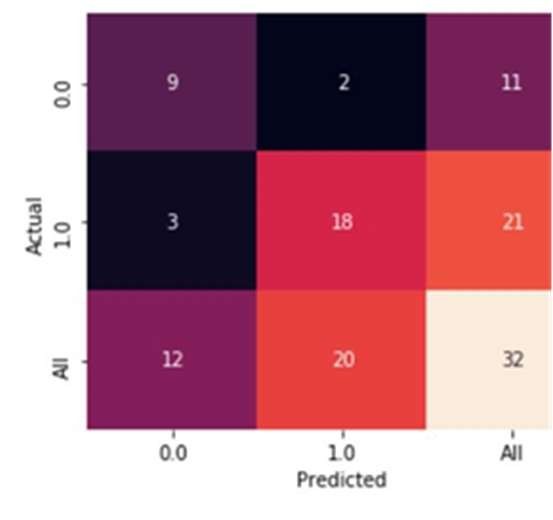
Figure 28. Confusion Matrix
TP = True Positives = 18; TN = True Negatives = 9; FP = False Positives = 3; FN = False Negatives = 2.
For correlation 2, the model yields a prediction accuracy of 75 %; the corresponding confusion matrix is shown in Figure 29.

Figure 29. Confusion Matrix
TP = True Positives = 19; TN = True Negatives = 5; FP = False Positives = 4; FN = False Negatives = 4.
For correlation 3, the model yields a prediction accuracy of 96,875 %; the corresponding confusion matrix is shown in Figure 30.

Figure 30. Confusion Matrix
TP = True Positives = 22; TN = True Negatives = 9; FP = False Positives = 4; FN = False Negatives = 0.
For correlation 4, the model yielded a prediction accuracy of 81,25 %; the corresponding confusion matrix is shown in Figure 31.

Figure 31. Confusion Matrix
TP = True Positives = 19; TN = True Negatives = 5; FP = False Positives = 4; FN = False Negatives = 4 .
Summary of Analysis
The summary of the analysis is captured as Table-1, wherein the respective correlations are plotted against their F1-scores.
|
Table 1. Results |
|||||
|
Model |
|
Accuracy |
Precision |
Recall |
F1 Score |
|
Backpropagation |
C1 |
0,94 |
0,95 |
095 |
0,95 |
|
|
C2 |
0,91 |
0,87 |
1,00 |
0,93 |
|
|
C3 |
0,97 |
0,96 |
1,00 |
0,98 |
|
|
C4 |
0,91 |
0,90 |
0,94 |
0,92 |
|
Recurrent Neural Network (GRU) |
C1 |
0,91 |
0,95 |
0,90 |
0,93 |
|
|
C2 |
0,84 |
0,86 |
0,91 |
0,89 |
|
|
C3 |
0,97 |
0,96 |
1,00 |
0,98 |
|
|
C4 |
0,81 |
0,90 |
0,82 |
0,86 |
|
|
|
|
|
|
|
|
K Nearest Neighbor |
C1 |
0,84 |
0,90 |
0,86 |
0,88 |
|
|
C2 |
0,75 |
0,83 |
0,83 |
0,82 |
|
|
C3 |
0,97 |
0,96 |
1,00 |
0,98 |
|
|
C4 |
0,81 |
0,85 |
0,85 |
0,85 |

Figure 32. Model performance comparison graph based on F1-score
ANALYSIS OF RESULTS
The objective of this study was to build a model that predicts Freshman student’s aptitude for computer programming using Machine learning algorithms. Several hypotheses were conjectured, and corresponding questionnaire generated; they were given to school final students in India and the dataset was collected.
Four models were built for each ANN based on four correlations generated using clustered hypotheses set; KNN was used as a classifier. The performance of the models was computed using the test dataset, which was 20 % of the original dataset. The results show that the BPN model/s achieved high accuracies in predicting the Freshman student’s aptitude for computer programming.
The best correlation scores for the clustered hypotheses C1, C2, C3 and C4 were 94 %, 91 %, 97 %, 91 % respectively. Although the best model was the BPN, it took the second longest time to train unlike the KNN, while the first being RNN. The results show that the models can be employed to predict Freshman student’s aptitude for programming. Further work in this arena include the use of Convolutional Neural Network (CNN) to study student’s aptitude for programming and also generate several useful 3-d metrics.
REFERENCES
1. Narasimhan L, Basupi G. Deep Learning Based Analysis of Student Aptitude for Programming at College Freshman Level 2023.
2. Longi K. Exploring factors that affect performance on introductory programming courses. Master thesis. University of Helsinki, 2016.
3. Ahadi A, Lister R, Haapala H, Vihavainen A. Exploring Machine Learning Methods to Automatically Identify Students in Need of Assistance. Proceedings of the eleventh annual International Conference on International Computing Education Research, New York, NY, USA: Association for Computing Machinery; 2015, p. 121–30. https://doi.org/10.1145/2787622.2787717.
4. Lakshmi Narasimhan V. Proactive Personalized Primary Care Information System (P3CIS). In: Kim H, Kim KJ, Park S, editors. Information Science and Applications, Singapore: Springer; 2021, p. 357–65. https://doi.org/10.1007/978-981-33-6385-4_33.
5. kumar VS, Narasimhan VL. Using Deep Learning For Assessing Cybersecurity Economic Risks In Virtual Power Plants. 2021 7th International Conference on Electrical Energy Systems (ICEES), 2021, p. 530–7. https://doi.org/10.1109/ICEES51510.2021.9383723.
6. Devasia T, P VT, Hegde V. Prediction of students performance using Educational Data Mining. 2016 International Conference on Data Mining and Advanced Computing (SAPIENCE), 2016, p. 91–5. https://doi.org/10.1109/SAPIENCE.2016.7684167.
7. Ward ME, Peters G, Shelley K. Student and Faculty Perceptions of the Quality of Online Learning Experiences. Irrodl 2010;11:57–77. https://doi.org/10.19173/irrodl.v11i3.867.
8. Kingma DP, Ba J. Adam: A Method for Stochastic Optimization 2017. https://doi.org/10.48550/arXiv.1412.6980.
9. Liu W, Wang Z, Yuan Y, Zeng N, Hone K, Liu X. A Novel Sigmoid-Function-Based Adaptive Weighted Particle Swarm Optimizer. IEEE Transactions on Cybernetics 2021;51:1085–93. https://doi.org/10.1109/TCYB.2019.2925015.
FINANCING
None
CONFLICT OF INTEREST
None
AUTHORSHIP CONTRIBUTION:
Conceptualization: V. Lakshmi Narasimhan, G. Basupi.
Investigation: V. Lakshmi Narasimhan, G. Basupi.
Writing – proofreading and editing: V. Lakshmi Narasimhan, G. Basupi.
|
APPENDIX-A: Questionnaire Employed |
|||||||||
|
Correlation |
Hypothesis |
Question |
Mean |
Mode |
Median |
Standard Deviation |
Rho |
Hypothesis Mean |
Hypothesis STD |
|
C1 |
0 |
1. I have enough skills to learn programming. |
3,8408 |
6 |
5 |
2,2773 |
0,23559 4 |
3,6943 |
2,3064 |
|
|
|
2. I have enough knowledge to learn programming |
3,5478 |
6 |
4 |
2,3355 |
0,26501 6 |
|
|
|
|
1 |
6. Computer programming Is difficult for me |
2,6752 |
1 |
2 |
2,1370 |
0,16288 4 |
2,6274 |
2,1621 |
|
|
|
7. Computer programming is not for me |
2,5796 |
1 |
1 |
2,1872 |
0,16888 2 |
|
|
|
|
2 |
12. I know some programming and hence learning formal programming is easy |
3,7898 |
6 |
5 |
2,3343 |
0,25157 9 |
3,3482 |
2,2713 |
|
|
|
13. I can program faster, because of past experience in programming |
3,4013 |
6 |
3 |
2,2613 |
0,24136 3 |
|
|
|
|
|
14. I do not like programming due to lack of experience with computer programming. |
2,8535 |
1 |
2 |
2,2183 |
0,18088 3 |
|
|
|
|
|
15. I have logical thinking skills and therefore programming is rather easy for me |
3,9873 |
6 |
5 |
2,1122 |
0,26297 7 |
3,3217 |
2,0810 |
|
|
3 |
16. I have difficulty in understanding logic and how it works and therefore I find programming difficult |
2,6561 |
1 |
2 |
2,0497 |
0,14113 3 |
|
|
|
|
5 |
20. I have the mental tenacity for handling difficult programming problems. |
2,9618 |
6 |
3 |
2,2699 |
0,19028 7 |
3,0573 |
2,2857 |
|
|
|
22. Mental tenacity has little relationship towards solving difficult programming problems |
3,1529 |
6 |
3 |
2,3015 |
0,19088 6 |
|
|
|
C2 |
6 |
23. Visual tools help me well in learning programming |
3,8344 |
6 |
5 |
2,3283 |
0,27401 2 |
3,0191 |
2,2104 |
|
|
|
24. I prefer pseudo code tools for learning programming |
2,7006 |
0 |
2 |
2,3300 |
0,23494 9 |
|
|
|
|
|
25. Visual tools are not helpful in learning/understanding of Programming |
2,5223 |
1 |
2 |
1,9728 |
0,21923 3 |
|
|
|
|
|
29. Gender of a person plays a role in learning programming |
2,2611 |
1 |
1 |
2,0790 |
0,16233 7 |
2,1943 |
2,0799 |
|
|
|
30. There exists gender bias in the process of learning |
2,1274 |
1 |
1 |
2,0808 |
0,19890 5 |
|
|
|
|
|
31. I learn programming better through visual environments. |
4,5159 |
6 |
6 |
2,4823 |
0,19694 9 |
4,1019 |
2,3727 |
|
C3 |
|
32. I learn programming better through collaborative learning environments |
3,8471 |
6 |
5 |
2,3593 |
0,18517 4 |
|
|
|
|
|
33. I prefer Visual environment for learning programming. |
3,9427 |
6 |
5 |
2,2765 |
0,26413 7 |
|
|
|
|
|
34. Female students learn programming better through visual environments |
2,8790 |
6 |
3 |
2,3543 |
0,15757 4 |
2,8599 |
2,3600 |
|
|
|
35. Female students learn programming better through collaborative learning environments. |
2,8408 |
6 |
3 |
2,3656 |
0,19214 9 |
|
|
|
|
9 |
37. Learning programming calls for minimum level of logical Skills. |
2,6752 |
0 |
2 |
2,1874 |
0,19111 7 |
2,8981 |
2,2249 |
|
|
|
39. learning programming calls for minimum level of logical skills. |
2,8981 |
6 |
3 |
2,1815 |
0,22464 2 |
|
|
|
C4 |
|
40. I have good degree of logical skills |
3,3503 |
6 |
4 |
2,2528 |
0,20306 3 |
|
|
|
|
|
41. I have good degree of experience in programming |
2,5796 |
1 |
2 |
2,1547 |
0,13783 5 |
|
|
|
|
|
42. I have good degree of mental tenacity |
2,9873 |
6 |
3 |
2,3479 |
0,15030 6 |
|
|
|
|
10 |
44. Learning programming calls for a cumulative minimum level in the sum of Logical Skills and Mental Tenacity. Below the cumulative levels, students get disinterested in learning computer programming |
2,5669 |
0 |
2 |
2,2454 |
0,10165 4 |
2,5669 |
2,2454 |
|
|
7 |
26. Collaborative learning environment helps me well in learning programming |
3,9427 |
6 |
5 |
2,4370 |
0,22260 6 |
3,4055 |
2,3572 |
|
|
|
27. I prefer collaborative learning environment for learning programming |
3,7516 |
6 |
5 |
2,3769 |
0,20388 |
|
|
|
|
|
28. collaborative learning environments are not helpful in learning/ understanding programming |
2,5223 |
0 |
2 |
2,2577 |
0,16232 9 |
|
|
APPENDIX-B: Brief Overview of the Algorithms Used
Multiple linear regression
Multi-Linear regression is the process of using many independent variables to deter- mine one dependent variable (many to 1 relationship). In Multiple Linear Regression, we try to find relationship between two or more independent variables (inputs) and corresponding dependent variable (output). The independent variables can be contin- uous or categorical.
Artificial neural network (ANN)
Artificial Neural Network (ANN) can be defined as information processing tools which mimic or copy the learning methodology of the biological neural networks. It derives its origin from the human nervous system, which consists of massively parallel large interconnection of large number of neurons, which activate different perceptual and recognition task in small amount of time. The last part of the research dealt with focusing on the use of my ANN to come up with a model that would predict student aptitude for programming based on the hypothesis elucidated in 3-Parameter Classification. For these four different models based on the correlation from each of the hypothesis were designed. The selected artificial neural networks are:
Backpropagation Neural Network (BNN)
Backpropagation is a feed forward neural network algorithm, which works by computing the gradient of the loss function with respect to each weight by the chain rule, computing the gradient one layer at a time, iterating backward from the last layer to avoid redundant calculations of intermediate terms in the chain rule. Backpropagation is a short form for "backward propagation of errors." It is a standard method of training artificial neural networks. This method helps to calculate the gradient of a loss function with respect to all the weights in the network.

Figure 33. Multilinear Regression Formula
Recurrent Neural Network (RNN) – Gated Recurrent Network
Recurrent Neural Network (RNN) is a type of Neural Network where the output from previous step is fed as input to the current step. In traditional neural networks, all the inputs and outputs are independent of each other. Thus, RNN came into existence, which solved this issue with the help of a Hidden Layer. The main and most important feature of RNN is Hidden state, which remembers some information about a sequence. They are especially powerful in use cases in which context is critical to predicting an outcome and are distinct from other types of artificial neural net- works because they use feedback loops to process a sequence of data that informs the final output, which can also be a sequence of data. The feedback loops allow information to persist; the effect is often described as memory. RNNs built with LSTM units categorize data into short term and long-term memory cells. Doing so enables RNNs to figure out data that is important and should be remembered and looped back into the network, and the data that can be forgotten or left out.
K-Nearest Neighbor
K-Nearest Neighbor (KNN) Algorithm uses the entire dataset in its training phase. Whenever a prediction is required for an unseen data instance, it searches through the entire training dataset for k-most similar instances and the data with the most similar instance is finally returned as the prediction. (Atul, 2020). Further, k-nearest neighbor algorithm uses a very simple approach to perform classification. When tested with a new example, it looks through the training data and finds the k-training examples that are closest to the new example.