Implication of Different Data Split Ratio on the Performance of Model in Price Prediction of Used Vehicles Using Regression Analysis

doi: 10.56294/dm2024425

ORIGINAL

Implication of Different Data Split Ratio on the Performance of Model in Price Prediction of Used Vehicles Using Regression Analysis

Repercusión de las distintas proporciones de división de datos en el rendimiento del modelo de predicción del precio de los vehículos usados mediante análisis de regresión

Alimul Haque¹ *, Shams Raza² *, Sultan Ahmad^3,4 *, Alamgir Hossain⁵ *, Hikmat A. M. Abdeljaber⁶ *, A.E.M. Eljialy⁷ *, Sultan Alanazi³ *, Jabeen Nazeer³ *

¹Department of Computer Science, Veer Kunwar Singh University. Ara, 802301, India.

²Academic Counselor, IGNOU International Division. India.

³Department of Computer Science, College of Computer Engineering and Sciences, Prince Sattam Bin Abdulaziz University. Alkharj, 11942, Saudi Arabia.

⁴School of Computer Science and Engineering, Lovely Professional University. Phagwara, 144411, Punjab, India.

⁵Department of Computer Science and Engineering, Prime University. Dhaka 1216, Bangladesh.

⁶Department of Computer Science, Faculty of Information Technology, Applied Science Private University. Amman, Jordan.

⁷Department of Information Systems, College of Computer Engineering and Sciences, Prince Sattam Bin Abdulaziz University. Alkharj, 11942, Saudi Arabia.

Cite as: Alimul Haque M, Shams Raza M, Ahmad S, Alamgir Hossain M, A. M. Abdeljaber H, M. Eljialy AE, et al. Implication of Different Data Split Ratios on the Performance of Models in Price Prediction of Used Vehicles Using Regression Analysis. Data and Metadata. 2024; 3:425. https://doi.org/10.56294/dm2024425

Submitted: 05-02-2024 Revised: 08-05-2024 Accepted: 11-07-2024 Published: 12-07-2024

Editor: Adrián Alejandro Vitón Castillo

ABSTRACT

Introduction: artificial intelligence (AI) and Machine Learning have become buzzwords lately due to technological changes and data quality testing, especially in shape and finish analysis. Lots of research has been conducted for linear regression algorithms to predict the price in different sectors for share stock, rental properties, prices of used cars etc. This study provides suitable data split ratio for optimum cost estimation based on linear regression model. In present days there is an increasing demand for having own car for every middle-class family therefore this have given opportunity to motor vehicle business to offer wide range of used vehicle for re-sale especially companies like Maruti Suzuki, Tata motors & Mahendra motors in Indian motor vehicle industries. Therefore, it is important to know the current value of your car before spending your hard-earned money on any item.

Objective: the objective of this paper is finding appropriate value of cars in Metropolitans or even in state capitals. Features like model, mileage, AC, seating capacities, fuel type automatic will be taken into account when doing this. This estimate is designed to help customers find the right options to suit their needs.

Method: we have used a linear regression model to estimate the value of the respective car.

Results: for doing this price prediction in this paper using liner regression we have tried to find the optimum accuracy of model by varying data split ratio for training and test data set and concluded with the result that 80/20 ratio is the best ratio with optimum model accuracy for business domain analysis with labelled data set.

Conclusions: the findings underscore the importance of careful consideration when selecting a data split ratio for price prediction models in the used vehicle market. The insights gleaned from this study can inform future research and contribute to the development of more accurate and reliable regression models in similar domains.

Keywords: Artificial Intelligence; Linear Models; Machine Learning; Commerce; Dataset.

RESUMEN

Introducción: la inteligencia artificial (IA) y el aprendizaje automático se han convertido últimamente en palabras de moda debido a los cambios tecnológicos y a la comprobación de la calidad de los datos, especialmente en el análisis de formas y acabados. Se ha investigado mucho sobre algoritmos de regresión lineal para predecir el precio en diferentes sectores para acciones, propiedades de alquiler, precios de coches usados, etc. Este estudio proporciona una relación de división de datos adecuada para la estimación óptima de costes basada en un modelo de regresión lineal. En la actualidad hay una creciente demanda de tener un coche propio para cada familia de clase media, por lo tanto, esto ha dado la oportunidad a las empresas de vehículos de motor para ofrecer una amplia gama de vehículos usados para la reventa, especialmente empresas como Maruti Suzuki, Tata Motors y Mahendra Motors en las industrias de vehículos de motor de la India. Por lo tanto, es importante conocer el valor actual de su coche antes de gastar su dinero duramente ganado en cualquier artículo.

Objetivo: el objetivo de este trabajo es encontrar el valor adecuado de los coches en Metropolitans o incluso en las capitales de los estados. Para ello, se tendrán en cuenta características como el modelo, el kilometraje, el aire acondicionado, la capacidad de los asientos y el tipo de combustible automático. Esta estimación está pensada para ayudar a los clientes a encontrar las opciones adecuadas a sus necesidades.

Método: hemos utilizado un modelo de regresión lineal para estimar el valor del coche correspondiente.

Resultados: para realizar esta predicción de precios en este artículo utilizando la regresión lineal, hemos intentado encontrar la precisión óptima del modelo variando la proporción de división de datos para el conjunto de datos de entrenamiento y de prueba, y hemos llegado a la conclusión de que la proporción 80/20 es la mejor con una precisión óptima del modelo para el análisis del dominio empresarial con un conjunto de datos etiquetados.

Conclusiones: los resultados subrayan la importancia de considerar cuidadosamente la selección de la proporción de datos para los modelos de predicción de precios en el mercado de vehículos usados. Las conclusiones de este estudio pueden servir de base para futuras investigaciones y contribuir al desarrollo de modelos de regresión más precisos y fiables en ámbitos similares.

Palabras clave: Inteligencia Artificial; Modelos Lineales; Aprendizaje Automático; Comercio; Conjunto de Datos.

INTRODUCTION

The most important issue when selling a vehicle is to determine the cheapest price and not to offer less than the value of the vehicle. If the bid price is higher than the market price, the car is less likely to sell or will take longer to sell. Also it is obvious from customer perspective that amount to be paid for the vehicle should be appropriate. Cost of a used vehicle will vary based on the vehicle’s attributes such as make of the car, year of make, mileage, glass quality, maintenance record, shades, comfort specifications. Harnessing all above information a machine learning model may be build for prediction of its sale price.

Machine learning is a process which is capable of solving a task by getting experience from training data and continuously improving itself for producing the results without involving programming instructions.^(1,2) So many studies had been done on application of machine learning algorithms into several areas of research and analysis for example COVID-19 analysis,^(2,3) crop identification,⁽⁴⁾ access to real-time predictions,⁽⁵⁾ and tracking of vehicle lost.⁽⁶⁾ In this paper we are using linear regression model for the price prediction. This model is having features of both statistical and machine learning. Objective of linear regression is to build a models that describe ideas and relationships between independent and dependent variables.⁽⁷⁾ Although there has been significant growth in machine learning algorithms research in the research field, surprisingly some proposals address performance evaluation across many aspects at design time. A few aspects in this regard are data split variance, size of sample datasets and selection of machine learning methods. Just to mention, a study comparing machine learning methods on digital terrain maps showed that model design and selection affects the output.^(8,9) The concept of data set portioning is breaking a single data set into two separate data set means bifurcating entire records into groups which training set for the training of the model and testing set for the validation of the model. Scholars have suggested for using the 70/30 or 80/20 (training/test) data split ratio for landslide damage problems.^{(10,11,12,13,14)} Concerning the product price prediction researchers have mostly used 70/30 ratio for building the machine learning models. Research shows that increasing the size of training materials improves learning outcomes and results in model stability. Increasing the training size from 30 % to 80 % for performance evaluation can improve test results. However, when the training size is increased from 80 % to 90 %, a difference emerges in the test. It is noticeable that the training data set size effects significantly on the performance of the models.⁽¹⁵⁾

The core objective of this paper is evaluation of models performance based on different data split ratio using used cars data set, and also to find the best split ratio for the model having optimum performance.

Research Contribution

AI and Machine learning consists sophisticated methods embedded in computing software which are design and implemented for solving the real-life problems.^(16,17,9) Major reason for using machine learning is its capability for analysing huge volume of data and deliver optimum results with quantifiable qualities.⁽¹⁸⁾ But it is a fact that its impact lies on the accuracy of data set and appropriate method of applying on the data set.⁽¹⁹⁾ Partitioning the dataset is important which responsible to deliver the view of data to the concerned analyst, therefore it is necessary to create a data benchmark which is essential to evaluate the effectiveness of the data set.^(20,21) Therefore, it is difficult to estimate the implication of data segmentation on the quality of machine learning models, which will lead to selecting appropriate data segmentation for better machine learning models. In this study, we have selected linear regression and optimized it with data split ratio for accuracy of modelling.

Data Set used

Data set name: cars_sales_data.csv

This dataset is taken from Kaggle data sets which contains used cars data and openly available. This dataset contains 8125 tuples and 16 features, having multiple brands Maruti, Honda, Toyota, Mahendra, Hyundai and Tata.

The dataset includes the following features: name, purchase year, sale price, running km, fuel, sold by gears, owners, mileage, engine, max_power, torque, seats, age.

This dataset can be used for multiple applications, such as:

· Market Analysis: analyzing the trends and patterns in the used car market based on factors like car type, year, and price.

· Pricing Insights: understanding the relationship between car specifications and pricing to assist in determining fair market value.

· Decision Making: supporting decisions related to car purchases, investments, and market strategies.

We have selected approx. 1600 rows and relevant features required for this research paper. The data set is presented in table 1 with few rows.

Table 1. Used Cars Data Set
Name	Year	Selling_Price	km_driven	Fuel	Transmission	Mileage	Engine	Seats	Age
Maruti Swift Dzire VDI	2014	450000	145500	Diesel	Manual	23,4 kmpl	1248 CC	5	7
Skoda Rapid 1.5 TDI Ambition	2014	370000	120000	Diesel	Manual	21,14 kmpl	1498 CC	5	7
Honda City 2017-2020 EXi	2006	158000	140000	Petrol	Manual	17,7 kmpl	1497 CC	5	15
Hyundai i20 Sportz Diesel	2010	225000	127000	Diesel	Manual	23,0 kmpl	1396 CC	5	11
Maruti Swift VXI BSIII	2007	130000	120000	Petrol	Manual	16,1 kmpl	1298 CC	5	14
Hyundai Xcent 1.2 VTVT E Plus	2017	440000	45000	Petrol	Manual	20,14 kmpl	1197 CC	5	4
Maruti Wagon R LXI DUO BSIII	2007	96000	175000	LPG	Manual	17,3 km/kg	1061 CC	5	14
Maruti 800 DX BSII	2001	45000	5000	Petrol	Manual	16,1 kmpl	796 CC	4	20
Toyota Etios VXD	2011	350000	90000	Diesel	Manual	23,59 kmpl	1364 CC	5	10
Ford Figo Diesel Celebration Edition	2013	200000	169000	Diesel	Manual	20,0 kmpl	1399 CC	5	8
Renault Duster 110PS Diesel RxL	2014	500000	68000	Diesel	Manual	19,01 kmpl	1461 CC	5	7
Maruti Zen LX	2005	92000	100000	Petrol	Manual	17,3 kmpl	993 CC	5	16
Maruti Swift Dzire VDi	2009	280000	140000	Diesel	Manual	19,3 kmpl	1248 CC	5	12

METHOD

Linear regression

Linear regression estimates the relationship between two variables by assuming a positive relationship between the individual variable and the dependent or target variable. It builds a straight line that minimized the equation between prediction and reality. This method is used to analyse and forecast different data in various fields such as business and finance. It can be extended to various types of linear and logistic regressions with many independent variables and is suitable for binary distribution problems.

Figure 1. Sample plotting of linear regression

In the above plot association between the Input (Independent variable) and the output (Dependent or target variable) has been expressed. The diagonal straight line (blue) is referred as best fit line covering average data points.

Metrics for Evaluation

For deciding the level of accuracy of linear regression model, it requires to measure it by means of some metrics.

Following are the two metrics we have used for this paper:

· Squared Correlation(R-Square)

· Root Mean Squared Error (RSME)

R-Square: this metrics reflects the variance percentage of selected input (independent) variables which are responsible for the prediction of target or dependent variable. It is expected that resultant value of R-Square should be at a higher level in a range of 0-1.

Its calculative equation may have expressed as: R² = 1 – (Un explain variation/ Total variation).

RMSE is one of the two performance metrics for linear regression. This metric compute the average difference between the predicted value by the model and the actual value of target variable. Finally, it discloses that accuracy of the model which is predicted near to real value.

Its calculative equation may have expressed as:

Tool: Rapid Miner

We have used Rapid Miner Studio 10.0 version for the implementation of our research. Big data analysts use platforms like Rapidminer and Data Scientist to quickly analyze and clean data before building good models. No coding or any type of knowledge is required to use Quickminer. Therefore, programmers to create smart models via logistic regression Rapidminer. It is also used by researchers. Rapid Miner provides data analysis, plugins, data analysis methods, etc. It has many tools and options for; this makes it compatible with web apps, mobile apps, Android and iOS apps and tools. It is also compatible with web tools like Flask, Node js, and can be used as cross-platform without the limitations of RapidMiner.

Implementation of research

Step-1

Data loading: using the Rapid miner interface we loaded the data set cars_sales_data.csv in the workflow window and checked the data view using data list tab. This is a label data set as it is a pre requisite for regression and classification analysis.

Step-2

Data Pre-processing: in the second step we have performed following data pre-processing task using the various Rapid miner operators.

Visualized the statistics of data which shows all details of the features such data type, missing value, range of data value, average value for each attributes or features.

Select initially required attributes.

Removed missing values using filter operator: convert the fuel attribute into three dummy attribute using Nominal to Numeric operator Petrol, Diesel, Cng.

Elimination of irrelevant Attributes using Select operator: we have eliminated few columns such as (Fuel Cng & Lpg), because the statistics have showed there is very few rows are having such value, and rows with minimal instance have no significance in regression analysis so it should be eliminated. Also we have eliminated (Year) as it does not have any significance for the price of car.

Finally, we have Selected the required columns for this task. As we are using linear regression model which required all the attribute should be numeric so we have selected following attributes:

1. Selling_price.

2. Km_driven.

3. Fuel_petrol.

4. Fuel_diesel.

5. Age.

6. Seat.

Finally, we have 6 attributes or features after selection and transformation and 1600 rows in our data set. Out of which one is our target variable or output variable (Selling_price) and others are treated as independent or input variable.

Step-3

Model building process: after getting the clean and optimized data we have performed following model building processes keeping the goal optimum selling_price prediction.

Specifying the Target Variable: we have marked our target or output variable as dependent variable (Price) using Set role operator, connecting with the selected data set.

Partitioning the data set into Training & Test data sets: we have divided the data set as training set and test set, using Split Data Operator, connecting with role specified data set.

This step we have repeated four times for changing the ratio of both Training and Test data after running and recording the result of each cycle of the regression analysis processes.

Additionally, missing value removal: before creation Linear regression model we have added Missing value operator as safety measure. Output port spline having label data of split data method is connected with its input port.

Creation of Linear Regression Model: we have created the Linear regression model using linear regression method. Then connected the training data spline(output) from missing value operator into its input port. This process (linear regression) generates the model as output which is supplied to Test process (Apply model) as input.

Creation of Test (Apply Model): we have created Model test process (Apply Model) by selecting Apply Model method from process tab. This process predict the values of the target variable based on the model supplied by regression model.

This process (Apply Model) is connected with the Test data spline (output) from split data processes into its second input port which is unlabelled or test data.

Then this process (Apply Model) is connect with the output spline(Model) of regression process (Regression Model) into its first input port which is the model.

This process generates two outputs first is the label data which is predicted values and second output is the model which used for prediction.

Creation of performance evaluation: in the final step we have added performance evaluation process (Regression Performance) by selecting regression performance metric from the process tab.

This process (Performance) evaluate the performance of the model and generate result. Also it generates sample predicted values for sharing with users.

The output spline of Apply model (Label) is connected to the input port of Performance (Label) and Output of performance port (Perform) & (Example) is send to result port.

Step-4

Execution of the process: after setting all above processes we have run the whole process and obtain output which are presented under result. In the final output port there are three splines which are presenting the overall results.

First spline (output) is from Performance evaluation process which presenting performance of the model in terms of multiple parameters, then values of RMSE (average predicted value +/-) & R-square (Correlation % of variance).

Second spline (output) is also from Performance evaluation process which is delivering continuous predicted values of the output variable along with actual input values.

Third spline (output) is from Apply model which is showing the mathematical equation of the model created by Regression Model. Overall Processes for linear regression analysis created under workflow of Rapid miner is given below.

Figure 2. Linear regression model building processes work flow diagram

We have run the above discussed linear regression process four times by changing the four different data split ratio, this has generated four different results for each execution cycle, these four results are presented in the result section for comparative analysis.

RESULTS

First Execution with 50-50 ratio and its Result

Actual price vs Predicted price

Figure 3. Sample Predicted Data

The output example set of first test is applied on sample data set of 1600 rows and continuous predicted values are generated for test data, it is presented in the figure 3 which is showing the very high predicted values in comparison to actual prices so this may not be a desired result with the applied data split 50-50 ratio for training data set and test data set.

Figure 4. Linear regression output

In the figure 4 the regression analysis output is presented which generated as result of First test applied with data set of 1600 rows and split 50-50 ratio. In this output two things Coefficient and P-value, are important related to selected independent variables such as in this case four variables fuel_Diesel, fuel_Petrol, km_driven and age.

In the above output values under coefficient reflects the impact of the variable on target variable in this case price, if the sign of the value is positive then it shows positive impact otherwise if it is negative then it reflects negative impact. Such as in this case other than fuel_Diesel all have negative impact on the target variable predicted price. Here in this output fuel_Petrol should not be negative.

Second thing in the above output is P-value, it is desirable that P-value should be less than 0,05 for each variable participated in prediction. In this output P-value of all the variables is within the range.

Performance Vector (Performance)

root_mean_squared_error: 886260,064 +/-

squared_correlation: 0,204

Above output of the First test for performance evaluation metrics of linear regression model has presented two values first is RMSE which is predicted price of the car which is very high in this output. Second is the value of R-square which reflecting the percentage variation of the variables participated in this model for prediction which is very low in this case. So both indicates the performance of the model is not optimum with 50-50 split ratio.

Model

244801,444 * fuel_Diesel

- 244799,062 * fuel_Petrol

- 3,817 * km_driven

- 64711,177 * age

+ 1341301,936

Above equation is the linear regression model build by the linear regression process based on 50-50 data split ratio in the First test.

Second Execution with 60-40 ratio and its Result

Actual price vs Predicted price

Figure 5. Sample Predicted Data

The example data set, output of Second test is presented in above figure 5 is having continuous predicted values along with actual prices. It is also showing the very high predicted values in comparison to actual prices so this may not be a desired result with the applied data split 60-40 ratio for training data set and test data set.

Figure 6. Linear regression output

In the above figure 6 the output of regression analysis is presented which is generated as result for Second test applied with data set of 1600 rows and split 60-40 ratio. In this output two things Coefficient and P-value are important related to selected independent variables such as in this case four variables fuel_Diesel, fuel_Petrol, km_driven and age.

In the above output values under coefficient reflects the impact of the variable on target variable in this case price, if the sign of the value is positive then it shows positive impact otherwise if it is negative then it reflects negative impact. Such as in this case two variables fuel_Diesel, fuel_Petrol have positive impact on the target variable predicted price and two variable km_driven, age have negative impact on the target variable predicted price. This output seems to be acceptable.

Second thing in the above output is P-value, it is desirable that P-value should be less than 0,05 for each variable participated in prediction. In this output P-value of two variables fuel_Diesel and fuel_Petrol is out of range and only two variables km_drive and age have their p-value within the range. So this output is not desirable.

Performance Vector (Performance)

root_mean_squared_error: 807596,682 +/-

squared_correlation: 0,239

Above output of the Second test for performance evaluation metrics of linear regression model has presented two values first is RMSE which is predicted price of the car which is very high in this output. Second is the value of R-square which reflecting the percentage variation of the variables participated in this model for prediction, which is very low in this case. So both indicates the performance of the model is not optimum with 60-40 split ratio.

Model

690851,136 * fuel_Diesel

+ 232693,023 * fuel_Petrol

- 3,945 * km_driven

- 68390,985 * age

+ 937151,578

Above equation is the linear regression model build by the linear regression process based on 60-40 data split ratio in the Second test.

Third Execution with 70-30 ratio and its Result

Actual price vs Predicted price

Figure 7. Sample Predicted Data

The example data set, output of Third test is presented in above figure 7 is having continuous predicted values along with actual prices. It is also showing the very high predicted values in comparison to actual prices so this may not be a desired result with the applied data split 70-30 ratio for training data set and test data set.

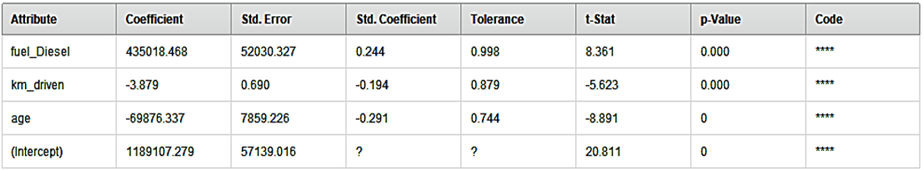
Figure 8. Linear regression output

In the above figure 8 the output of regression analysis is presented which is generated as result for Third test applied with data set of 1600 rows and split 70-30 ratio. In this output two things Coefficient and P-value are important related to selected independent variables such as in this case only three variables fuel_Diesel, km_driven and age.

In the above output values under coefficient reflects the impact of the variable on target variable in this case price, if the sign of the value is positive then it shows positive impact otherwise if it is negative then it reflects negative impact. Such as in this case one variables fuel_Diesel, have positive impact on the target variable’s predicted price and two variable km_driven, age have negative impact on the target variable’s predicted price so this output may be acceptable.

Second thing in the above output is P-value, it is desirable that P-value should be less than 0,05 for each variable participated in prediction. In this output P-value of all three variables are have their P-value within the range so this output may be acceptable.

Performance Vector (Performance)

root_mean_squared_error: 795037,551 +/-

squared_correlation: 0,254

Above output of the Third test for performance evaluation metrics of linear regression model has presented two values first is RMSE which is predicted price of the car which is very high in this output. Second is the value of R-square which reflecting the percentage variation of the variables participated in this model for prediction, which is very low in this case. So both indicates the performance of the model is not optimum with 70-30 split ratio.

Model

435018,468 * fuel_Diesel

- 3,879 * km_driven

- 69876,337 * age

+ 1189107,279

Above equation is the linear regression model build by the linear regression process based on 70-30 data split ratio in the Third test.

Fourth Execution with 80-20 ratio and its Result

Actual price vs Predicted price

Figure 9. Sample Predicted Data

The example data set, output of Fourth test is presented in above figure 9 which is having continuous predicted values along with actual prices. It is showing comparatively moderate predicted values in comparison to actual prices so this is a desired result with the applied data split 80-20 ratio for training data set and test data set.

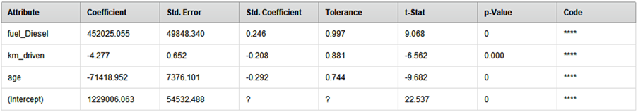
Figure 10. Linear regression output

In the figure 10 the output of regression analysis is presented which is generated as result for Fourth test applied with data set of 1600 rows and split 80-20 ratio. In this output two parameters, Coefficient and P-value are important related to selected independent variables such as in this case three variables fuel_Diesel, km_driven and age.

In the output values under coefficient reflects the impact of the variable on target variable in this case price, if the sign of the value is positive then it shows positive impact otherwise if it is negative then it reflects negative impact. Such as in this case one variables fuel_Diesel, have positive impact on the target variable’s predicted price and two variable km_driven, age have negative impact on the target variable’s predicted price so this output may be acceptable.

Performance Vector (Performance)

root_mean_squared_error: 717413,364 +/-

squared_correlation: 0,275

Above output of the Fourth test for performance evaluation metrics of linear regression model has presented two values first is RMSE which is predicted price of the car which is very appropriate in this output. Second is the value of R-square which reflecting the percentage variation of the variables participated in this model for prediction, which is comparatively high in this case. So both indicates the performance of the model is optimum with 80-20 split ratio.

Model

452025,055 * fuel_Diesel

- 4,277 * km_driven

- 71418,952 * age

+ 1229006,063

Above equation is the linear regression model build by the linear regression process based on 80-20 data split ratio in the Fourth test.

Comparative result Analysis

Data set sample size in each Test = 1600 rows.

Table 1. Integrated Results of all the four test cycle
Test cycle	Split ratio	Attributes	Coefficient	P-Value	P-Value < or > 0,05	RMSE	R-square
		fuel_Diesel	244801,444	2,42E-05	<0,05
First	50-50	fuel_Petrol	-244799,062	2,42E-05	<0,05	886260,064 +/-	0,204
		km_driven	-3,81673481	9,64E-11	<0,05
		age	-64711,177	8,88E-16	<0,05
		fuel_Diesel	690851,1364	0,07907	>0,05
Second	60-40	fuel_Petrol	232693,0225	0,554956	>0,05	807596,682 +/-	0,239
		km_driven	-3,94509315	7,20E-08	<0,05
		age	-68390,9847	1,22E-15	<0,05
		fuel_Diesel	435018,468	2,22E-16	<0,05
Third	70-30	fuel_Petrol				795037,551 +/-	0,254
		km_driven	-3,87883006	2,39E-08	<0,05
		age	-69876,337	0	<0,05
		fuel_Diesel	452025,055	0	<0,05
Fourth	80-20	fuel_Petrol				717413,364 +/-	0,275
		km_driven	-4,27668267	7,80E-11	<0,05
		age	-71418,9516	0	<0,05

In the above table 1 we have presented the integrated results of all the four tests based on required parameters. In this comparative output the result of fourth test is clearly showing the performance of linear regression model based on 80-20 ratio is optimum.

DISCUSSION

The investigation into the implication of various data split ratios on the performance of models in the price prediction of used vehicles through regression analysis underscores several key insights.

In the above test results it is clearly observed that optimum accuracy of model depends of the following five factors:

1. Sample set of predicted price against actual price.

2. Impact of independent variables in the model as coefficient.

3. P-value shows the significance of attributes participated in model (desirable is less than 0,05).

4. RMSE which is actual predicted price by the model with a little variation +/- (It should be win-win for both buyer and seller).

5. Square correlation required value is nearer to 1 which shows percentage of variance of the participating attributes in the prediction of price by the model (higher value is better)

As above in the comparative analysis we have found that value of RMSE predicted price is appropriate and comparatively lowest of all the four results, also the value of R-square is comparatively highest in all the four tests. These two factors are sufficient to prove that 80-20 split ratio is best for the optimum accuracy of the model. Therefore, after comparing all the five factors of above referred four tests it is clearly proved that data split ratio 80-20 is the best ratio for generation of accurate liner regression model for predictive analysis of labelled data set to obtained optimum accurate result. Overall, the findings underscore the importance of careful consideration when selecting a data split ratio for price prediction models in the used vehicle market. The insights gleaned from this study can inform future research and contribute to the development of more accurate and reliable regression models in similar domains.

ACKNOWLEDGMENT

We thank the Deanship of Scientific Research, Prince Sattam Bin Abdulaziz University, Alkharj, Saudi Arabia for help and support. This study is supported via funding from Prince Sattam Bin Abdulaziz University project number (PSAU/2024/R/1445).

BIBLIOGRAPHIC REFERENCES

1. S. Zeba, M. A. Haque, S. Alhazmi, and S. Haque, “Advanced Topics in Machine Learning,” Mach. Learn. Methods Eng. Appl. Dev., p. 197, 2022.

2. V. Whig, B. Othman, A. Gehlot, M. A. Haque, S. Qamar, and J. Singh, “An Empirical Analysis of Artificial Intelligence (AI) as a Growth Engine for the Healthcare Sector,” in 2022 2nd International Conference on Advance Computing and Innovative Technologies in Engineering (ICACITE), IEEE, 2022, pp. 2454–2457.

3. M. A. Haque et al., “Achieving Organizational Effectiveness through Machine Learning Based Approaches for Malware Analysis and Detection,” Data Metadata, vol. 2, p. 139, 2023.

4. D. Sinwar, V. S. Dhaka, M. K. Sharma, and G. Rani, “AI-based yield prediction and smart irrigation,” in Internet of Things and Analytics for Agriculture, Volume 2, Springer, 2020, pp. 155–180.

5. I. Hapsari and I. Surjandari, “Visiting time prediction using machine learning regression algorithm,” in 2018 6th International Conference on Information and Communication Technology (ICoICT), IEEE, 2018, pp. 495–500.

6. N. Nafi’iyah and K. F. Mauladi, “Linear regression analysis and SVR in predicting motor vehicle theft,” in 2021 International Seminar on Application for Technology of Information and Communication (iSemantic), IEEE, 2021, pp. 54–58.

7. M. Kavita and P. Mathur, “Crop yield estimation in India using machine learning,” in 2020 IEEE 5th International Conference on Computing Communication and Automation (ICCCA), IEEE, 2020, pp. 220–224.

8. S. Ahmad, S. Jha, A. Alam, M. Yaseen, and H. A. M. Abdeljaber, “A Novel AI-Based Stock Market Prediction Using Machine Learning Algorithm,” Sci. Program., vol. 2022, 2022.

9. M. A. Hossain et al., “AI-enabled approach for enhancing obfuscated malware detection: a hybrid ensemble learning with combined feature selection techniques,” Int. J. Syst. Assur. Eng. Manag., 2024, doi: 10.1007/s13198-024-02294-y.

10. D. T. Bui, B. Pradhan, O. Lofman, I. Revhaug, and O. B. Dick, “Landslide susceptibility mapping at Hoa Binh province (Vietnam) using an adaptive neuro-fuzzy inference system and GIS,” Comput. Geosci., vol. 45, pp. 199–211, 2012.

11. W. Chen et al., “Landslide susceptibility modelling using GIS-based machine learning techniques for Chongren County, Jiangxi Province, China,” Sci. Total Environ., vol. 626, pp. 1121–1135, 2018.

12. F. Huang, K. Yin, J. Huang, L. Gui, and P. Wang, “Landslide susceptibility mapping based on self-organizing-map network and extreme learning machine,” Eng. Geol., vol. 223, pp. 11–22, 2017.

13. K. Taalab, T. Cheng, and Y. Zhang, “Mapping landslide susceptibility and types using Random Forest,” Big Earth Data, vol. 2, no. 2, pp. 159–178, 2018.

14. N. N. Vasu and S.-R. Lee, “A hybrid feature selection algorithm integrating an extreme learning machine for landslide susceptibility modeling of Mt. Woomyeon, South Korea,” Geomorphology, vol. 263, pp. 50–70, 2016.

15. C. Qi, A. Fourie, Q. Chen, and Q. Zhang, “A strength prediction model using artificial intelligence for recycling waste tailings as cemented paste backfill,” J. Clean. Prod., vol. 183, pp. 566–578, 2018.

16. J. Zhou, P. G. Asteris, D. J. Armaghani, and B. T. Pham, “Prediction of ground vibration induced by blasting operations through the use of the Bayesian Network and random forest models,” Soil Dyn. Earthq. Eng., vol. 139, p. 106390, 2020.

17. S. Lu, M. Koopialipoor, P. G. Asteris, M. Bahri, and D. J. Armaghani, “A novel feature selection approach based on tree models for evaluating the punching shear capacity of steel fiber-reinforced concrete flat slabs,” Materials (Basel)., vol. 13, no. 17, p. 3902, 2020.

18. J. Qiu, Q. Wu, G. Ding, Y. Xu, and S. Feng, “A survey of machine learning for big data processing,” EURASIP J. Adv. Signal Process., vol. 2016, no. 1, 2016, doi: 10.1186/s13634-016-0355-x.

19. H.-B. Ly, B. T. Pham, L. M. Le, T.-T. Le, V. M. Le, and P. G. Asteris, “Estimation of axial load-carrying capacity of concrete-filled steel tubes using surrogate models,” Neural Comput. Appl., vol. 33, pp. 3437–3458, 2021.

20. M, Iyyappan, Ahmad S, Jha S, Alam A, Yaseen M, Abdeljaber HA., “A Novel AI-Based Stock Market Prediction Using Machine Learning Algorithm” Scientific Programming. Article ID 4808088, 11 pages, 2022

21. I. Muraina, “Ideal dataset splitting ratios in machine learning algorithms: general concerns for data scientists and data analysts,” in 7th International Mardin Artuklu Scientific Research Conference, 2022, pp. 496–504.

FUNDING

This study is supported via funding from Prince Sattam Bin Abdulaziz University project number (PSAU/2024/R/1445).

CONFLICT OF INTEREST

The authors declare that they have no known competing financial interests or personal relationships that could have appeared to influence the work reported in this paper.

AUTHOR CONTRIBUTIONS

Conceptualization: Alimul Haque, Shams Raza, Sultan Ahmad, Alamgir Hossain.

Investigation: Alimul Haque, Shams Raza, Sultan Ahmad, Alamgir Hossain, Sultan Alanazi.

Methodology: Alimul Haque, Shams Raza, Sultan Ahmad, Alamgir Hossain, A.E.M. Eljialy, Hikmat A. M. Abdeljaber, Jabeen Nazeer.

Writing - original draft: Alimul Haque, Shams Raza, Sultan Ahmad, Alamgir Hossain, A.E.M. Eljialy, Hikmat A. M. Abdeljaber, Sultan Alanazi, Jabeen Nazeer.

Writing - review and editing: Alimul Haque, Shams Raza, Sultan Ahmad, Alamgir Hossain, Sultan Alanazi, Hikmat A. M. Abdeljaber, A.E.M. Eljialy, Jabeen Nazeer.